
Skip to content

CFD Time Step Calculator: Courant (CFL) Number and Δt for Transient Simulations

Choosing the time step is one of the first decisions in any transient CFD simulation, and one of the easiest to get wrong. Too large, and the solution becomes unstable or smears out the unsteady features you are trying to capture. Too small, and the run takes days longer than it needs to. The Courant number, also called the CFL number, links the time step to the mesh and the flow velocity and gives a reliable starting point.

This free CFD time step calculator estimates Δt from a target Courant number, then checks it against optional limits that often matter more: the acoustic Courant number in compressible flow, the diffusion number for explicit schemes, and the number of time steps needed to resolve a known frequency such as vortex shedding. It also estimates the flow-through time, the number of time steps and the wall-clock time, so you can see what a run will cost before you launch it.

For a feel of the physics that a well-chosen time step must capture, the flow over a cylinder visualisation shows how vortex shedding develops as the Reynolds number changes.

Quick answer

A starting time step for transient CFD is Δt = C · Δx / U, where C is the target Courant number, Δx the smallest cell size in the region of interest and U the local flow velocity. For example, with U = 10 m/s, Δx = 0.5 mm and C = 1, Δt = 50 µs.

Treat this as a first estimate based on one representative velocity and cell size. Your solver calculates a local Courant number in every cell from the face fluxes, cell geometry and its own definition, so the maximum it reports can be noticeably higher, especially in small, stretched or skewed cells. The final time step also depends on the solver, the discretisation, the physics and the temporal resolution you need, so confirm it with a time-step sensitivity study.
Jump to the time step calculator ↓


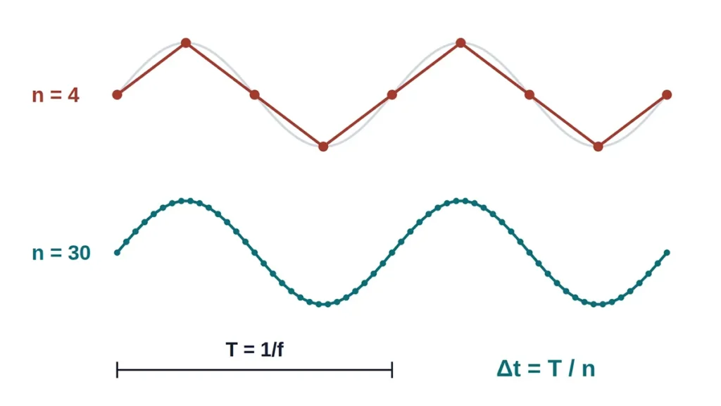
A periodic signal captured with 4 and with 30 time steps per period, showing the time step needed for temporal resolution

CFD Time Step Calculator (Courant / CFL Number)

Estimate a starting time step for a transient CFD simulation from the convective Courant number, then check it against optional acoustic, diffusion and temporal-resolution limits. The calculator also estimates the number of time steps, simulated time and run time.

1. Flow and Mesh

2. Additional Limits (optional)

3. Run Length and Cost (optional)

Time Step Results

Recommended time step—
Rounded time step—
Courant number (estimate)—
Total time steps—
Flow-through time, L/U—
Simulated physical time—
Steps per period—
Estimated wall-clock time—
ConstraintFormulaΔt limitValue at recommended ΔtValue at rounded Δt
Time step limits by constraint (log scale)
Unsure whether your transient model resolves the physics, or need a full time-step and mesh sensitivity study? Ask CFD Vision about transient CFD support.
Method: Δt = C·Δx/|U| (convective Courant number); Δt = Ca·Δx/(|U| + c) (acoustic); Δt = d·Δx²/ν or d·Δx²/α (explicit diffusion number, momentum or heat); Δt = 1/(n·f) with f = St·U/D (temporal resolution). The recommended value is the smallest active limit; the rounded value is the next lower 1–2–2.5–5 number. Courant numbers here use one representative U and Δx; a solver computes local values in every cell from face fluxes and cell geometry, using its own definition, so its reported maximum can differ. This is a preliminary estimate: the appropriate time step depends on the solver (explicit or implicit), the spatial and temporal discretisation, the transient physics and the required temporal resolution, and should be confirmed with a time-step sensitivity study.
');w.document.close();w.focus();setTimeout(function(){w.print();},300); }$('tsCalc').addEventListener('click',calc); $('tsReset').addEventListener('click',reset); $('tsPrint').addEventListener('click',printDoc); $('tsCsv').addEventListener('click',csv); $('tsPng').addEventListener('click',chartPng); reset(); })();

What the CFD Time Step Calculator Does

The calculator treats time-step selection as a set of competing limits and reports which one governs, rather than relying on the Courant number alone.

  • Convective Courant number limit from velocity, cell size and your target Courant number.
  • Optional acoustic Courant number limit for compressible flow, based on the flow velocity plus the speed of sound.
  • Optional diffusion number limit for explicit treatment of viscous (ν) or thermal (α) diffusion, with the stability limit set by the number of dimensions.
  • Optional temporal-resolution limit from a known frequency or a Strouhal number and body size.
  • The governing time step, a rounded value that is easy to enter in a solver, and the resulting Courant, acoustic and diffusion numbers.
  • Flow-through time, steps per flow-through, total steps, simulated time and estimated wall-clock time, with a chart and PDF, CSV and PNG exports.

You can also enter a specific time step that you already use, and the calculator shows the Courant number and other dimensionless numbers it produces.


What Is the Courant (CFL) Number?

The Courant number compares how far the flow travels in one time step with the size of a cell:

C=U ΔtΔx⇒Δt=C ΔxUC = \frac{U\,\Delta t}{\Delta x} \quad\Rightarrow\quad \Delta t = \frac{C\,\Delta x}{U}

A Courant number of 1 means fluid crosses one cell per time step. The condition is named after Courant, Friedrichs and Lewy, who showed in 1928 that an explicit scheme becomes unstable when information travels further than its numerical stencil can follow in one step. For an explicit solver, keeping C at or below a scheme-dependent limit, typically around 1, is therefore a stability requirement.

Implicit solvers, which most commercial pressure-based codes use for unsteady flow, remain stable at larger Courant numbers. Even so, accuracy still depends on it, because large time steps smear vortices, fronts and other moving features. In practice, the Courant number becomes a resolution criterion rather than a stability limit.

Which Velocity and Cell Size Should You Use?

The Courant number varies from cell to cell, and the maximum value usually matters most. For a conservative estimate, use the highest velocity together with the smallest cells in the region where the transient features occur, such as a jet, a wake or a shear layer. Using the mean inlet velocity and an average cell size can underestimate the local Courant number by an order of magnitude.

Even with good inputs, the calculator gives an estimate, not the value your solver will report. CFD codes calculate the Courant number cell by cell from the face fluxes and the cell volume, and their definitions differ, for example in how the velocity components or face fluxes in a 3D cell are combined. On stretched, skewed or polyhedral cells the reported maximum can therefore be noticeably higher than U·Δt/Δx. Check the Courant number your solver reports after the first time steps and adjust Δt if needed.


Choosing a Target Courant Number

There is no single correct Courant number. The values below are common starting points that practitioners then refine through a time-step sensitivity study and the guidance of their solver documentation.

Simulation typeCommon starting Courant numberMain reason
Explicit time integrationAt or below about 1, depending on the schemeNumerical stability
Implicit URANS, pressure-basedAbout 1 to 5 in the region of interestAccuracy of unsteady features
LES and scale-resolving DESAbout 1 or lower in the resolved regionResolving turbulent eddies in time
Free-surface VOFOften 0.25 to 1, based on the interfaceKeeping the interface sharp and bounded

Other Limits on the Time Step

Acoustic Courant Number in Compressible Flow

In a compressible solver, pressure waves travel at the speed of sound relative to the flow, so the relevant wave speed is |U| + c. At low Mach number this limit is far stricter than the convective one: at 10 m/s in air, it is about 35 times smaller. Unless acoustics matter to the result, a pressure-based or low-Mach-number formulation with implicit time integration avoids paying for it.

Δt≤Ca Δx|U|+c\Delta t \le \frac{C_a\,\Delta x}{|U| + c}

Diffusion Number for Explicit Schemes

When diffusion is treated explicitly, stability also requires a bounded diffusion number d = Γ Δt / Δx², where Γ is the diffusivity of the equation concerned: the kinematic viscosity ν for momentum and the thermal diffusivity α = k/(ρcp) for heat. For the classic explicit central scheme with equal spacing, the limit is 1/(2 × number of dimensions): 0.5 in one dimension, 0.25 in two and 1/6 in three, so a 1D value of 0.5 is not safe for a 3D calculation. For gases ν and α are similar (Prandtl number about 0.7). In water α is about seven times smaller than ν, so the momentum limit usually governs, while in liquid metals the thermal limit governs. Because it scales with Δx², this limit becomes severe on fine near-wall meshes, which is one reason most general-purpose CFD codes treat diffusion implicitly.

Temporal Resolution of the Physics

A stable time step is not necessarily an accurate one. To capture a periodic phenomenon, you need enough steps per period. For vortex shedding, the frequency follows from the Strouhal number, f = St · U / D, and St is close to 0.2 for a circular cylinder over a wide range of subcritical Reynolds numbers. Practitioners commonly use between 20 and 100 time steps per period, with the higher end when accurate amplitudes, phase or higher harmonics matter.


How Long Should a Transient Simulation Run?

The time step tells you how fine the time grid must be, while the run length decides how much physical time you must cover. A useful unit is the flow-through time, L / U, the time a fluid particle takes to cross the domain. Initial transients usually need a few flow-through times to wash out, and statistics such as mean drag or RMS pressure then need many more periods to converge.

Once you know the number of time steps, the wall-clock time follows from the cost per step, including the inner iterations of an implicit solver. Seeing that figure early is often what prompts a sensible compromise between mesh resolution, time step and run length.

Time-Step Independence

Just as a mesh study checks spatial discretisation, a time-step study checks temporal discretisation. Run the case with at least two, and ideally three, time steps that differ by a constant factor, keep the mesh fixed, and compare the quantities of interest once their statistics have converged. The mesh independence (GCI) calculator applies equally to the time-step size.

Common Mistakes When Choosing a Time Step

  • Basing the Courant number on the mean velocity and average cell size instead of local maxima.
  • Assuming an implicit solver makes the time step irrelevant to accuracy.
  • Too few inner iterations per time step, so that each step is not converged before the solver moves on.
  • Starting statistics before the initial transient has washed out, or stopping before enough periods have been averaged.
  • Refining the mesh without reducing the time step, which raises the Courant number in the refined region.

Transient CFD rewards experience, particularly for LES, multiphase or rotating machinery. CFD Vision provides transient CFD analysis services for industry, and CFD training and academic support for researchers who want to set up time-accurate simulations with confidence.


Frequently Asked Questions

What is a good CFL number for CFD?

For explicit schemes, the Courant number usually has to stay at or below about 1 for stability, and the exact limit depends on the scheme. Implicit solvers tolerate higher values, but a Courant number of around 1 in the region of interest is a sound starting point when unsteady features matter.

Can I use any time step with an implicit solver?

An implicit solver may remain stable, but a large time step damps and distorts the unsteady flow. The result can look smooth and converged while missing the physics, so accuracy still has to be checked with a time-step study.

How many time steps per period do I need?

Commonly between 20 and 100 time steps per period of the dominant frequency. Fewer steps can capture the frequency approximately, while accurate amplitudes, phases and harmonics need more.

Why does my transient simulation diverge?

Common causes include a local Courant number far above the intended value in small cells, poor mesh quality, too few inner iterations per time step, unsuitable initial conditions, and aggressive under-relaxation or scheme settings. Reducing the time step is a useful diagnostic, but it rarely fixes a mesh-quality problem on its own.

Should I use adaptive time stepping?

Adaptive time stepping based on a maximum Courant number is useful when velocities change strongly during the run, such as at start-up or in sloshing and filling. For statistically steady flows, a fixed time step often makes post-processing and frequency analysis simpler.


References

  • Courant, R., Friedrichs, K. and Lewy, H. (1928). Über die partiellen Differenzengleichungen der mathematischen Physik. Mathematische Annalen, 100, 32–74.
  • Ferziger, J. H., Perić, M. and Street, R. L. (2020). Computational Methods for Fluid Dynamics, 4th edition. Springer.
  • Celik, I. B. et al. (2008). Procedure for estimation and reporting of uncertainty due to discretization in CFD applications. Journal of Fluids Engineering, 130(7), 078001.

Planning a transient CFD study?

Send your case description to [email protected] for advice on time step, mesh and run length, or a complete transient CFD analysis. CFD Vision can sign an NDA before you share any files.

More free tools: engineering calculators for heat transfer, fluid flow and CFD, including the Reynolds number calculator and the y+ and first-cell height calculator.