
Skip to content

CFD Mesh Independence Calculator: Grid Convergence Index (GCI) and Richardson Extrapolation

Every CFD result carries a discretisation error, because the governing equations are solved on a finite mesh rather than in a continuum. A mesh independence study, more precisely a mesh convergence study, estimates how large that error is and whether further refinement would still change the answer. Reviewers, clients and thesis examiners increasingly expect to see one, and the grid convergence index (GCI) has become the most widely used way to report it.

This free CFD mesh independence calculator applies the GCI procedure published by Celik et al. in the Journal of Fluids Engineering, based on the original method of Roache. You enter the cell counts and results from three systematically refined meshes, and it returns the observed order of accuracy, the Richardson-extrapolated value, the GCI, the convergence type and a verdict against your target uncertainty for each monitored quantity. It even estimates how many cells you would need to reach your target uncertainty.

The calculator reproduces the published worked example of Celik et al. exactly, so you can check the implementation yourself before trusting it with your own study. Because the mesh near walls strongly affects wall-bounded results, the first-cell height and y+ calculator is a useful companion when you build the mesh family.
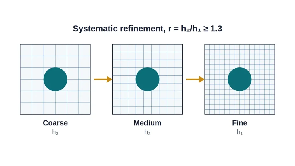
Coarse, medium and fine CFD meshes showing systematic refinement for a mesh independence study

Quick answer

In practice, “mesh-independent” means that further refinement no longer changes the quantity of interest by more than an acceptable amount. No mesh study proves this outright; it provides evidence of mesh convergence and an estimate of the remaining discretisation uncertainty. To estimate it, solve the same case on three systematically refined meshes, check that the results converge monotonically, and calculate the grid convergence index: GCI = 1.25 · ea / (rp − 1), where ea is the relative change between the two finest meshes, r is the refinement ratio and p is the observed order of accuracy.

The GCI is a percentage uncertainty band on the fine-mesh result due to discretisation alone.
Jump to the mesh independence calculator ↓


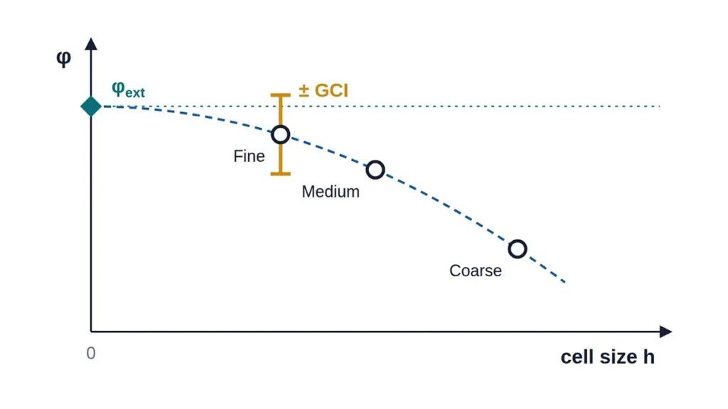
Solution plotted against cell size, showing Richardson extrapolation to zero cell size and the GCI uncertainty band

CFD Mesh Independence Calculator (GCI)

Enter results from three systematically refined meshes to get the observed order of accuracy, Richardson-extrapolated value, grid convergence index (GCI) and convergence type for each monitored quantity, following the procedure of Celik et al. (2008). Two meshes are also accepted, giving a two-mesh estimate with an assumed order and a safety factor of 3 rather than the three-grid GCI.

1. Meshes

Mesh 1 is the finest. Use the total cell count of each mesh, or a representative cell size if you know it. Refinement should be systematic, ideally with a refinement ratio above 1.3 between meshes.

2. Monitored Quantities

Add each quantity you monitored, such as a force coefficient, pressure drop, heat transfer rate or a probe velocity. Leave the coarse-mesh value blank to use the two-mesh estimate.

Mesh Convergence Results

Refinement ratio r21—
Refinement ratio r32—
Quantities assessed—
Within target—
QuantityChange 2→1Change 3→2ConvergenceObserved order pExtrapolated valueUncertaintyStatus
Standard GCIfine—
Conservative screening estimate—
Extrapolated value φext—
Asymptotic range check—≈ 1 when in asymptotic range
Solution versus relative cell size
Results not converging, oscillating, or needing an independent verification and validation review? Talk to a CFD specialist about your mesh study.
Method: Celik et al. (2008), J. Fluids Eng. 130(7), 078001, based on Roache’s grid convergence index. h ∝ N−1/D; observed order p from the three solutions by fixed-point iteration; Richardson extrapolation φext = (r21pφ1 − φ2)/(r21p − 1); GCIfine = 1.25·ea/(r21p − 1). Two-mesh results are outside the three-grid procedure: they assume the formal order and use Fs = 3, following Roache’s recommendation when the observed order cannot be verified. The conservative screening estimate is an additional heuristic used by this calculator, not part of the Celik et al. procedure: it takes p = min(observed p, formal order) and uses Fs = 3 unless the observed order is within 10% of the formal order. The verdict is based on the standard GCI, not on the screening estimate. GCI estimates discretisation uncertainty only; it does not include iteration error, modelling error or validation against experiment.
');w.document.close();w.focus();setTimeout(function(){w.print();},300); }$('mgAddQ').addEventListener('click',function(){addQ();}); $('mgCalc').addEventListener('click',calc); $('mgReset').addEventListener('click',reset); $('mgPrint').addEventListener('click',printDoc); $('mgCsv').addEventListener('click',csv); $('mgPng').addEventListener('click',chartPng); reset(); })();

What the Mesh Independence Calculator Does

For each quantity you monitor, the calculator works through the full GCI procedure and reports the results in a form you can paste straight into a report or paper.

  • Refinement ratios between the meshes, calculated from cell counts and problem dimension, or from cell sizes directly.
  • Percentage change between successive meshes and the convergence type: monotonic, oscillatory or divergent.
  • Observed order of accuracy, compared with the formal order of your numerical scheme.
  • Richardson-extrapolated value, approximate and extrapolated relative errors, and the fine-mesh GCI.
  • An asymptotic range check, a separate conservative screening estimate and, where needed, an estimate of the cell count that would meet your target.
  • A chart of the solution against relative cell size with the extrapolated value and uncertainty band, plus PDF, CSV and PNG exports.

Since different quantities converge at different rates, you can assess several at once. In practice, an integral quantity such as drag often converges well before a local quantity such as peak wall temperature or a velocity at a probe point, so it pays to check both.


How to Run a Mesh Independence Study

The arithmetic is the easy part. A trustworthy study depends far more on how the meshes are built and how each case is solved.

  1. Build at least three meshes with systematic refinement. Keep the topology, growth rates and refinement regions consistent, so that the meshes differ mainly in cell size.
  2. Use a refinement ratio of at least 1.3 between successive meshes, as Celik et al. recommend. Smaller ratios make the result sensitive to iteration error and round-off.
  3. Keep the physics, boundary conditions, schemes and solver settings identical on every mesh. In particular, avoid switching between wall functions and a resolved boundary layer as y+ changes.
  4. Converge every case tightly. The iteration error should be much smaller than the difference between meshes, otherwise the study measures solver noise rather than discretisation error.
  5. Monitor the quantities that matter to the decision you are making, including at least one integral and one local quantity.
  6. Report the cell counts, refinement ratios, observed order, extrapolated values and GCI for each quantity.

The Grid Convergence Index Method Step by Step

The calculator follows the five-step procedure of Celik et al. (2008). First, a representative cell size is defined for each mesh. For a mesh of N cells in D dimensions:

h∝N−1/D,r21=h2h1=(N1N2)1/Dh \propto N^{-1/D},\quad r_{21} = \frac{h_2}{h_1} = \left(\frac{N_1}{N_2}\right)^{1/D}

Next, with ε21 = φ2 − φ1 and ε32 = φ3 − φ2, the observed order p is found by fixed-point iteration from:

p=1ln⁡r21|ln⁡|ε32ε21|+q(p)|,q(p)=ln⁡(r21p−sr32p−s)p = \frac{1}{\ln r_{21}}\left|\ln\left|\frac{\varepsilon_{32}}{\varepsilon_{21}}\right| + q(p)\right|,\quad q(p) = \ln\left(\frac{r_{21}^p – s}{r_{32}^p – s}\right)

Here, s = sign(ε32/ε21). When the two refinement ratios are equal, q = 0 and p follows directly. The extrapolated value then estimates the solution at zero cell size:

φext21=r21pφ1−φ2r21p−1\varphi_{\mathrm{ext}}^{21} = \frac{r_{21}^p\varphi_1 – \varphi_2}{r_{21}^p – 1}

Finally, the approximate relative error and the fine-mesh grid convergence index are:

ea21=|φ1−φ2φ1|,GCIfine21=1.25 ea21r21p−1e_a^{21} = \left|\frac{\varphi_1 – \varphi_2}{\varphi_1}\right|,\quad \mathrm{GCI}_{\mathrm{fine}}^{21} = \frac{1.25\, e_a^{21}}{r_{21}^p – 1}

The factor 1.25 is a safety factor recommended when three or more meshes confirm the observed order. With only two meshes, the order cannot be checked, so the calculator falls back to the formal order and a safety factor of 3, following Roache’s recommendation.


How to Interpret the Convergence Type

The ratio R = ε21/ε32 describes how the solution behaves as the mesh is refined, and it decides whether Richardson extrapolation is meaningful.

Ratio RConvergence typeWhat it means
0 < R < 1Monotonic convergenceThe change shrinks steadily with refinement. Richardson extrapolation and the GCI apply.
−1 < R < 0Oscillatory convergenceThe solution overshoots and undershoots but the swings shrink. The calculator reports half the range of the three solutions as the uncertainty instead.
R > 1Monotonic divergenceThe change grows with refinement. The meshes are not converging, so no uncertainty can be estimated.
R < −1Oscillatory divergenceGrowing oscillation between meshes. Check mesh quality, iterative convergence and the refinement strategy.

Observed Order and the Asymptotic Range

Richardson extrapolation assumes the meshes lie in the asymptotic range, where the discretisation error falls in proportion to hp. A strong sign that this holds is an observed order close to the formal order of the scheme, which is usually 2 for a second-order finite-volume method. If the observed order is far lower, the coarse mesh is probably too coarse. If it is far higher, errors from different sources may be cancelling, and the GCI may be optimistic.

The calculator also reports Roache’s asymptotic range check, GCI32 / (r21p · GCI21), which should be close to 1. Alongside the standard GCI, it shows a conservative screening estimate. This is a heuristic used by this calculator, not part of the Celik et al. three-grid procedure: it takes p as the smaller of the observed and formal orders, and applies a safety factor of 3 instead of 1.25 when the observed order differs from the formal order by more than 10%. Use it as a sensitivity check when the evidence for asymptotic behaviour is weak, and report the standard GCI as your main result. The factor of 3 is also used for two-mesh estimates, following Roache’s recommendation when the observed order cannot be verified; it is not the three-grid GCI factor.


What a Mesh Independence Study Does Not Tell You

The GCI quantifies discretisation uncertainty and nothing else. A solution with a small GCI can still be wrong if the turbulence model, boundary conditions, material properties or geometry do not represent reality. For that reason, verification answers the question “are we solving the equations correctly?”, while validation against experimental data answers “are we solving the right equations?”.

Likewise, the GCI does not include iteration error or, in transient simulations, time-step error. For unsteady cases, a separate time-step independence study is needed, and the CFD time step calculator helps you choose a sensible starting time step for it.

Common Mistakes in Mesh Studies

  • Refining only part of the domain, so that the meshes are not a systematic family.
  • Using refinement ratios close to 1, which amplifies noise in the observed order.
  • Stopping iterations too early, so that the iteration error is comparable with the mesh-to-mesh change.
  • Changing the near-wall treatment between meshes because y+ moves across the wall-function range.
  • Judging independence from a single global quantity while the decision depends on a local value.
  • Declaring independence from two meshes that happen to agree, without a third mesh to confirm the trend.

If your study shows oscillation, divergence or an implausible order, an experienced reviewer can usually find the cause quickly. CFD Vision provides CFD analysis services for industry, and CFD training and academic support for researchers and students preparing verification evidence for a thesis or paper.


Frequently Asked Questions

What GCI value is acceptable?

There is no universal threshold. The acceptable uncertainty depends on how the result will be used: a design comparison between two concepts can tolerate more than a result used to certify a margin. Many engineering studies aim for a GCI of a few percent on the key quantities, which is why the calculator lets you set your own target.

How many meshes do I need for a mesh independence study?

Three is the minimum to estimate the observed order of accuracy and check the convergence type. Two meshes only give an estimate based on an assumed order with a larger safety factor, and a fourth mesh adds confidence when the results are noisy or the order is uncertain.

What refinement ratio should I use between meshes?

Celik et al. recommend a refinement ratio greater than 1.3. In 3D, a ratio of 1.3 corresponds to about 2.2 times as many cells, and a ratio of 2 to eight times as many, so the finest mesh often sets the practical limit.

Why is my observed order much higher or lower than 2?

Usually because the meshes are not yet in the asymptotic range, the refinement was not systematic, the iterations were not fully converged, or different error sources partly cancel. Mixed first- and second-order schemes, limiters and wall functions can also reduce the observed order.

Does a mesh-independent solution mean the CFD result is correct?

No. A small GCI is evidence that the estimated discretisation uncertainty is small for that quantity, but it is an estimate, not proof, and modelling assumptions can still produce a wrong answer. Validation against experimental or trusted reference data is needed to judge physical accuracy.

Can I use the GCI for transient simulations?

Yes. The same procedure applies to a time-averaged quantity or to the time-step size in a time-step independence study, provided the other parameters are held constant and the statistics are converged.


References

  • Celik, I. B., Ghia, U., Roache, P. J., Freitas, C. J., Coleman, H. and Raad, P. E. (2008). Procedure for estimation and reporting of uncertainty due to discretization in CFD applications. Journal of Fluids Engineering, 130(7), 078001.
  • Roache, P. J. (1994). Perspective: a method for uniform reporting of grid refinement studies. Journal of Fluids Engineering, 116(3), 405–413.
  • Roache, P. J. (1998). Verification and Validation in Computational Science and Engineering. Hermosa Publishers.
  • ASME V&V 20-2009. Standard for Verification and Validation in Computational Fluid Dynamics and Heat Transfer.

Need confidence in your CFD results?

Send your case description to [email protected] for an independent review of your mesh study, a full verification and validation plan, or a complete CFD analysis. CFD Vision can sign an NDA before you share any files.

More free tools: engineering calculators for heat transfer, fluid flow and CFD, including the y+ and first-cell height calculator and the Reynolds number calculator.