
A heat exchanger transfers thermal energy between two fluids at different temperatures while normally preventing direct mixing between the streams. As a result, heat exchangers are fundamental components in HVAC systems, power generation, chemical processing, refrigeration, electronics cooling, energy recovery, automotive thermal management, data centers, and many other industrial applications.
For preliminary engineering analysis, the Heat Exchanger Calculator on this page provides an estimate of heat exchanger performance and sizing. Specifically, it combines the effectiveness–NTU method, logarithmic mean temperature difference (LMTD), energy balances, and optional internal-flow calculations to estimate heat duty, outlet temperatures, effectiveness, required heat-transfer area, Reynolds number, Nusselt number, convection coefficients, pressure losses, and hydraulic pumping power.
The calculator is particularly useful during preliminary engineering and before detailed CFD simulation and CFD consulting are undertaken. Analytical calculations can establish expected operating ranges, while CFD can subsequently investigate three-dimensional flow distribution, thermal gradients, recirculation, local pressure losses, flow maldistribution, and geometric effects that simplified calculations cannot resolve.
Quick answer
Heat duty: Q = ε · Cmin · (Th,in − Tc,in) with the effectiveness–NTU method, or Q = U · A · ΔTlm with the LMTD method, where Cmin is the smaller heat-capacity rate (ṁcp) and NTU = UA / Cmin.
Use effectiveness–NTU when outlet temperatures are unknown (performance rating), and LMTD when the target duty and temperatures are known and you need the required area (sizing).
Heat Exchanger Performance & Design Calculator
Analyse ideal counterflow or parallel-flow heat exchangers using effectiveness–NTU and LMTD methods. Estimate heat duty, outlet temperatures, required area, effectiveness, and optional simplified tube/channel thermal-hydraulic performance.
Hot Side
Stream HCold Side
Stream CHeat Exchanger Definition
This optional module is intended for preliminary analysis of straight circular tubes or approximate hydraulic-diameter passages. It assumes equal mass-flow distribution across all parallel passages.
Hot-Side Passage
Cold-Side Passage
Thermal Resistance Additions
Heat Exchanger Results
Temperature Change Across Each Stream
Thermal Analysis
| Parameter | Result |
|---|---|
| Hot heat-capacity rate | — |
| Cold heat-capacity rate | — |
| Cmin / Cmax ratio | — |
| Maximum possible duty | — |
| Hot-side temperature change | — |
| Cold-side temperature change | — |
Design Interpretation
| Parameter | Result |
|---|---|
| Flow configuration | — |
| Calculation method | — |
| Minimum capacity stream | — |
| Minimum terminal approach | — |
| Temperature cross | — |
What Does the Heat Exchanger Calculator Calculate?
The calculator provides two primary calculation modes.
Performance Analysis — Known U and Heat-Transfer Area
If the overall heat-transfer coefficient and heat-transfer area are known, the calculator uses the effectiveness–NTU method to determine:
- heat-transfer rate,
- hot-side outlet temperature,
- cold-side outlet temperature,
- heat exchanger effectiveness,
- number of transfer units (NTU),
- LMTD,
- heat-capacity rates,
- maximum theoretical heat-transfer rate.
This mode is useful when evaluating an existing exchanger or estimating the performance of a proposed exchanger with approximately known and .
Heat Exchanger Sizing — Known Target Heat Duty
If the required heat duty and a design value of are known, the calculator estimates the heat-transfer area required to achieve that duty under the specified ideal flow arrangement.
This can provide a useful first-stage sizing estimate before detailed exchanger design, experimental validation, or CFD-based product development.
An optional hydraulic module extends the calculation to Reynolds number, Prandtl number, Nusselt number, convection coefficients, Darcy friction factor, pressure drop, and hydraulic pumping power for tube-like or channel-like passages.
Fundamental Heat Exchanger Energy Balance
For a steady-state heat exchanger with negligible heat loss to the surroundings, the heat removed from the hot stream is equal to the heat gained by the cold stream.
For the hot fluid:
For the cold fluid:
where:
= heat-transfer rate
= mass flow rate
= specific heat capacity at constant pressure
= fluid temperature
Subscripts and represent the hot and cold streams respectively.
These relationships are the basic conservation-of-energy equations behind the calculator.
For constant fluid properties and no phase change, they allow the outlet temperatures to be determined once the heat-transfer rate is known.
Heat-Capacity Rates in Heat Exchanger Analysis
The heat-capacity rate of each fluid is:
and
The minimum and maximum heat-capacity rates are then:
The heat-capacity-rate ratio is:
This ratio is important because the two streams do not necessarily respond equally to the same heat-transfer rate.
For example, a stream with a relatively low heat-capacity rate undergoes a larger temperature change for a given than a stream with a high heat-capacity rate.
Maximum Possible Heat Transfer and Heat Exchanger Effectiveness
The maximum theoretical heat-transfer rate is obtained by allowing the fluid with the minimum heat-capacity rate to approach the inlet temperature of the opposite stream.
Therefore:
Heat exchanger effectiveness is defined as:
The effectiveness therefore indicates how closely the exchanger approaches the maximum thermodynamically possible heat transfer for the specified inlet conditions and flow rates.
For example, an effectiveness of means that the exchanger transfers 75% of the maximum possible heat transfer available under those inlet conditions.
Effectiveness is useful for comparing heat exchangers because it normalizes actual performance against the theoretical maximum.
The Effectiveness–NTU Method for Heat Exchanger Performance
The number of transfer units is defined as:
where:
= overall heat-transfer coefficient
= effective heat-transfer area
= smaller heat-capacity rate
NTU represents the thermal size of the heat exchanger relative to the ability of the fluid streams to carry heat.
Generally, increasing increases NTU and therefore increases exchanger effectiveness, although the relationship is nonlinear and depends on the heat-capacity-rate ratio and flow configuration.
Parallel-Flow Heat Exchanger Effectiveness
For an ideal parallel-flow heat exchanger:
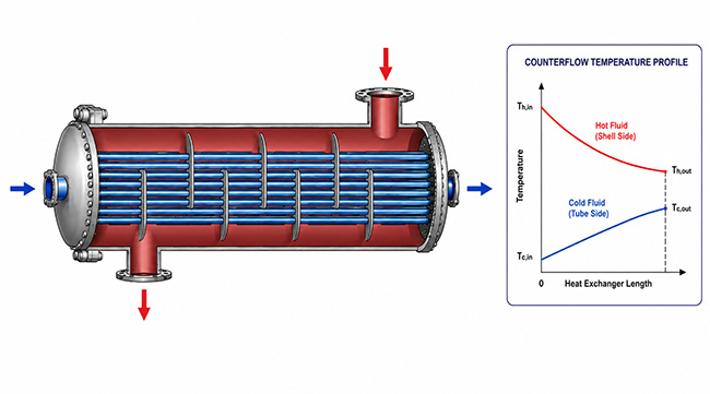
In parallel flow, both fluids enter the exchanger from the same end and travel in the same overall direction.
The temperature difference between the fluids is therefore greatest at the inlet and progressively decreases along the exchanger.
Counterflow Heat Exchanger Effectiveness
For an ideal counterflow heat exchanger and :
When:
the expression becomes:
Counterflow arrangements can generally achieve greater effectiveness than comparable parallel-flow arrangements because a useful temperature difference can be maintained over more of the exchanger length.
LMTD Method for Heat Exchanger Design
Another fundamental heat exchanger relationship is:
where is the logarithmic mean temperature difference.
It is calculated from:
For an ideal counterflow exchanger:
For an ideal parallel-flow exchanger:
When the required heat duty and overall heat-transfer coefficient are known, the required area can be estimated from:
This is the basis of the calculator’s sizing mode.
For complex shell-and-tube arrangements, crossflow exchangers, multipass exchangers, and other non-ideal configurations, appropriate correction factors or configuration-specific methods may be required. The simple parallel-flow and counterflow equations should not be interpreted as universal models for every exchanger geometry.
Can the Cold Outlet Be Hotter Than the Hot Outlet?
This is an important point because the result can initially appear physically impossible.
Consider a counterflow heat exchanger with:
and
For the calculator’s example conditions of approximately:
with water-like heat capacities, the calculation gives approximately:
and
Thus:
This is not automatically an error.
In an ideal counterflow heat exchanger, the hot and cold outlet temperatures occur at opposite physical ends of the exchanger. The cold outlet is locally adjacent to the hot inlet region rather than the hot outlet region.
Therefore, the relevant terminal temperature differences are approximately:
and
Both remain positive.
Consequently, a cold-stream outlet temperature higher than the hot-stream outlet temperature can be physically valid in counterflow operation.
The same temperature cross is not compatible with an ideal parallel-flow exchanger because both streams travel in the same direction and their temperature profiles cannot cross under the assumptions used here.
Optional Hydraulic Analysis for CFD and Thermal Engineering
Thermal performance alone does not determine whether a heat exchanger is practical.
Increasing velocity can improve convective heat transfer, but it usually also increases pressure losses and pumping requirements. Heat exchanger design therefore involves a trade-off between thermal performance and hydraulic performance.
The optional hydraulic section of the calculator estimates these effects for idealized tube-like or channel-like passages.
Reynolds Number in Heat Exchanger Flow
The Reynolds number is:
where:
= fluid density
= mean flow velocity
= hydraulic diameter
= dynamic viscosity
Reynolds number indicates the relative importance of inertial and viscous effects and is fundamental to determining internal-flow behaviour.
For conventional internal flows, low Reynolds numbers are associated with laminar behaviour, while sufficiently high Reynolds numbers generally correspond to turbulent flow. The intermediate region requires particular care.
If you want to examine Reynolds number independently, CFD Vision also provides a Reynolds Number Calculator.
Prandtl Number and Thermal Boundary-Layer Behaviour
The Prandtl number is defined as:
where is the fluid thermal conductivity.
Prandtl number compares momentum diffusivity with thermal diffusivity and therefore plays an important role in convective heat-transfer correlations.
The relationship between Reynolds number, Prandtl number, Nusselt number, wall conditions, and geometry ultimately determines the convective heat-transfer coefficient.
Nusselt Number and Convection Coefficient
The Nusselt number is defined as:
Therefore:
where is the convective heat-transfer coefficient.
For fully developed laminar flow in a circular tube with constant wall temperature, a classical result is:
This value should not be treated as universally applicable to every laminar heat exchanger passage. Different wall boundary conditions, developing flow, non-circular geometries, and entrance effects can produce different Nusselt numbers.
For additional heat-transfer calculations, the Nusselt Number Calculator for Convective Heat Transfer provides a useful companion tool.
Gnielinski Correlation for Turbulent Heat Transfer
For suitable turbulent internal-flow conditions, the calculator uses the Gnielinski correlation:
where is the Darcy friction factor.
The Gnielinski correlation is widely used for turbulent forced convection in internal flows, but like all empirical correlations it has a defined applicability range. It should not simply be extrapolated to arbitrary Reynolds numbers, Prandtl numbers, geometries, or strongly developing flows.
The calculator therefore identifies transitional conditions as preliminary estimates rather than implying that a simple correlation precisely predicts the physics in this region.
Churchill Friction Factor for Pressure-Loss Estimation
The calculator uses the Churchill correlation for the Darcy friction factor.
One useful feature of the Churchill formulation is that it provides a continuous expression covering laminar, transitional, and turbulent internal-flow conditions while accounting for relative surface roughness.
The Darcy friction factor can then be used with the Darcy–Weisbach equation:
where:
= Darcy friction factor
= passage length
= hydraulic diameter
= fluid density
= mean velocity
The calculator estimates straight-passage friction losses. Losses associated with headers, manifolds, bends, entrances, exits, contractions, expansions, fittings, and other geometric features are not included.
For a more focused pipe-flow calculation, see CFD Vision’s Hydraulic Pressure Drop Calculator.
Hydraulic Pumping Power
The ideal hydraulic power associated with the calculated pressure loss is:
where is the volumetric flow rate.
Actual electrical or shaft power will be greater because real pumps and drive systems have efficiencies below 100%.
For example, if pump efficiency is represented by , a simplified shaft-power estimate would be:
The calculator reports hydraulic power before pump efficiency is applied.
Estimating the Overall Heat-Transfer Coefficient
When the optional convection analysis is enabled, the calculator also produces a simplified resistance-based estimate of the overall heat-transfer coefficient:
where:
= hot-side convection coefficient
= cold-side convection coefficient
= hot-side fouling resistance
= cold-side fouling resistance
= wall thermal resistance
This simplified resistance model is useful for preliminary engineering calculations.
However, actual exchanger design may require careful treatment of the area basis, tube-wall geometry, cylindrical conduction, fins, contact resistance, fouling, material properties, and exchanger configuration. Therefore, the estimated should not automatically be treated as a manufacturer-grade design value.
For conduction and convection through multiple thermal resistances, the Multi-Layer Total Heat Transfer Coefficient Calculator provides additional calculations.
Why Analytical Heat Exchanger Calculations Are Not Enough
Analytical methods are extremely valuable because they are fast, transparent, and suitable for preliminary sizing and performance checks.
However, most real heat exchangers contain three-dimensional flow phenomena that cannot be represented completely by one-dimensional engineering correlations.
Examples include:
- nonuniform flow distribution between tubes or channels,
- header and manifold losses,
- recirculation regions,
- separation,
- local jets,
- bypass flow,
- dead zones,
- nonuniform wall heat flux,
- conjugate heat transfer,
- local hot spots,
- complex turbulence,
- geometry-dependent pressure losses.
The calculator assumes that total mass flow is divided evenly among parallel passages. Real heat exchanger headers may produce significant flow maldistribution.
That is precisely where CFD simulation services can extend preliminary analytical calculations.
Heat Exchanger CFD Simulation
In a detailed CFD model, the governing conservation equations are solved throughout the computational domain rather than reducing the exchanger to average inlet and outlet quantities.
For fluid flow, the continuity equation can be written as:
The momentum equations may be represented as:
and the energy equation provides the basis for predicting the spatial thermal field.
Instead of producing only a single pressure-drop or outlet-temperature value, CFD can provide fields of:
and
This makes it possible to identify the physical mechanisms responsible for exchanger performance.
For engineers interested in the broader relationship between numerical simulation and thermal engineering, Advanced CFD Thermal Management Solutions for Heat Control discusses applications of CFD to thermal-management problems.
Heat Exchangers in Industrial CFD Applications
Heat exchanger performance is important across many engineering sectors.
For HVAC applications, coils and heat-recovery systems must achieve the required thermal performance while controlling fan and pumping energy.
Data centers present another challenge because heat rejection and cooling equipment interact with airflow distribution throughout the facility. Therefore, CFD can connect equipment-level thermal performance with room-level airflow and temperature management. CFD Vision discusses this application further in The Role of CFD Simulations in Data Centers for Optimum Cooling and Energy Saving.
Meanwhile, in industrial process systems, pressure loss can be as important as heat-transfer performance. Excessive pressure drop can increase operating costs even when the exchanger achieves the required thermal duty.
In product development, simulation can be used to investigate alternative channel arrangements, header geometries, flow rates, materials, and thermal configurations before physical prototypes are manufactured. This simulation-driven approach is discussed further in CFD in Product Development: From Engineering Concept to Simulation-Driven Design.
From Heat Exchanger Calculations to CFD Consulting
A calculator and a CFD model answer different engineering questions.
The calculator is appropriate for questions such as:
“What heat duty should this exchanger approximately achieve?”
“What outlet temperatures should I expect?”
“How much heat-transfer area might be required?”
“What is the approximate Reynolds number?”
“What pressure loss should a straight passage produce?”
A CFD model becomes more useful when the questions become:
“Why are some channels receiving less flow?”
“Where is the pressure loss actually occurring?”
“Which regions have poor heat transfer?”
“Is the header causing maldistribution?”
“Where are the thermal hot spots?”
“How would a geometry modification affect both heat transfer and pressure drop?”
For such problems, computational fluid dynamics consulting can provide information that a lumped engineering model cannot.
This distinction is important: simple analytical models should not be replaced unnecessarily by CFD, but CFD should also not be replaced by simplified correlations when local three-dimensional physics determine the design outcome.
Important Engineering Assumptions
Results from this calculator should be interpreted as preliminary engineering estimates.
The principal assumptions include steady-state operation, constant representative fluid properties, no phase change, negligible external heat loss, ideal parallel-flow or counterflow behaviour, and simplified tube/channel hydraulics.
For the optional hydraulic calculations, the total flow rate is assumed to divide equally among the specified parallel passages.
The laminar result:
assumes fully developed internal flow with constant wall temperature.
The Churchill correlation provides a continuous Darcy friction-factor estimate across flow regimes, however the convective heat-transfer treatment of the transitional Reynolds-number range remains inherently more uncertain.
The calculator therefore bridges the laminar and turbulent Nusselt-number treatments in the transitional region as an engineering approximation rather than claiming a universally validated transitional heat-transfer model.
Similarly, straight-passage pressure drop does not include local losses produced by headers, bends, fittings, entrances, exits, contractions, expansions, or other exchanger-specific geometry.
Scientific Basis and Further Reference
The heat exchanger relationships used here are standard results from convective heat-transfer and thermal-engineering theory. The effectiveness–NTU method, LMTD method, internal-flow Nusselt correlations, and heat exchanger energy balances are discussed extensively in established heat-transfer literature.
A useful external engineering reference is the MIT Unified Engineering thermodynamics and heat-transfer material, which provides university-level background on thermodynamics and heat-transfer principles.
The Gnielinski turbulent heat-transfer correlation originates from V. Gnielinski’s work on heat transfer in tubes, while the continuous Darcy friction-factor formulation used by the calculator is based on Churchill’s 1977 correlation.
These analytical methods remain extremely useful for preliminary engineering, but correlation validity, boundary conditions, geometry, property variation, and flow regime should always be considered when interpreting the result.
Using the Calculator as Part of an Engineering Workflow
A practical heat exchanger development workflow can begin with analytical calculations to establish approximate thermal duty, outlet temperatures, heat-transfer area, pressure drop, and expected flow regime.
Those calculations can then define realistic operating conditions for detailed simulation.
CFD can subsequently evaluate the geometry under those conditions, identify limitations, and support design modifications. Promising configurations can then be validated experimentally or against operational measurements.
This creates a useful engineering progression:
For engineers and researchers developing their own simulation capabilities, CFD Vision also provides CFD training and ANSYS Fluent support.
Conclusion
The Heat Exchanger Performance & Design Calculator provides a practical bridge between fundamental heat-transfer theory and more advanced thermal-fluid analysis. It can estimate heat duty, effectiveness, NTU, LMTD, outlet temperatures, required heat-transfer area, Reynolds and Prandtl numbers, Nusselt number, convection coefficients, pressure drop, and hydraulic pumping power.
These calculations are valuable for preliminary sizing, engineering checks, educational analysis, and establishing realistic starting conditions for more detailed simulations.
For real heat exchangers, however, average analytical values cannot describe every aspect of the internal flow and temperature fields. Flow maldistribution, header design, recirculation, local pressure losses, conjugate heat transfer, complex geometry, and nonuniform thermal behaviour may require detailed numerical investigation.
When those effects become important, CFD Vision provides CFD consulting and CFD analysis services for industrial thermal-fluid problems, helping connect fundamental engineering calculations with detailed simulation and design optimization.
Related Engineering Calculators
Continue your analysis with the other free engineering calculators from CFD Vision:
Check whether a flow is laminar, transitional or turbulent for common gases, water or custom fluids.
Nusselt number and convective heat transfer coefficient from standard internal and external flow correlations.
Multi-Layer Heat Transfer Coefficient Calculator
Overall U-value and total thermal resistance for walls with conduction, contact resistance and convection.
Pipe Flow Pressure Drop Calculator
Darcy-Weisbach pressure loss, friction factor and flow regime for liquid flow in pipes.
CFD Y+ and First-Cell Height Calculator
Estimate the first-cell height for a target y+ before building inflation layers in your CFD mesh.
Flow Over a Cylinder Visualization
Interactive view of boundary-layer separation, wake formation and vortex shedding as Reynolds number changes.
Need More Than a Hand Calculation?
For flow maldistribution, header design, fouling-sensitive geometry or conjugate heat transfer, our CFD simulation and analysis services resolve what average correlations cannot. For CFD consulting services and thermal design support, visit our main page or read About CFD Vision.